Any system or process can be described by some mathematical equations. Their nature may be arbitrary. Does security service of a stadium want to know fan traffic in the case of fire? Does an engineer construct a thermal generating unit for your house? Usually, using a small set of general rules and laws of nature, one can predict everything at least for the nearest future. So, in this article, we’ll continue our topic of the computer simulations and deal with the way all these calculations are performed.
Let us consider the following problem: how to hit a target in a given position with a canon? This problem has a simple analytical solution, so it will be easy to check ourselves. Let the cannon be placed in the origin, i.e. its horizontal coordinate is x_c=0 and the vertical coordinate is the same, y_c=0. This pair is an initial coordinate of a missile:
x(t=0)=0, \ y(t=0)=0
A cannon can fire a missile with the initial velocity v_0 at the angle of \alpha to the horizon. Its motion is determined by gravity. The Newton’s second law gives us all equations needed:
m\vec{a} = \vec{F}
There is only an acceleration g=9.81\ \dfrac{m}{s^2} due to the gravity directed downside: a_y=-g. And the horizontal motion is steady, i.e. a_x=0. Thus, the force \vec{F} = -mg\hat{y} with \hat{y} being the unit vector in the vertical direction. It results in the following system of equations:
<br /> \begin{cases}<br /> ma_x = 0\\<br /> ma_y = -mg\\<br /> \end{cases}\implies\begin{cases}<br /> a_x = 0\\<br /> a_y = -g\\<br /> \end{cases} (1)
Below, we show a simple numerical solution of this problem using python. Our physical background is given by the Eqns (1) and one needs to integrate them. To do this, we define a class [python]Cannon[/python] with the constructor, accepting initial parameters:
[python]class Cannon:def __init__(self, x0, y0, v, angle):
    """
    x0 and y0 are initial coordinates of the cannon
    v is the initial velocity
    angle is the angle of shooting in degrees
    """
    # current x and y coordinates of the missile
    self.x    = x0
    self.y    = y0
    # current value of velocity components
    self.vx  = v*cos(radians(angle))
    self.vy  = v*sin(radians(angle))

    # acceleration by x and y axes
    self.ax   = 0
    self.ay   = -9.8
    # start time
    self.time = 0

    # these list will contain discrete set of missile coordinates
    self.xarr = [self.x]
    self.yarr = [self.y]
[/python]
The simplest integration may be constructed in the following way. After a short period of time \Delta t, velocity v is changed by \Delta v = a \Delta t:
v(t+\Delta t) = v(t) + a\Delta t
The corresponding methods for calculation of v_x(t) and v_y(t) are:
[python]    def updateVx(self, dt):
        self.vx = self.vx + self.ax*dt
        return self.vx
    def updateVy(self, dt):
        self.vy = self.vy + self.ay*dt
        return self.vy
[/python]
A small shift of a missile in space can be calculated as a motion with an average velocity \dfrac{v(t) + v(t+\Delta t)}{2}:
[python]    def updateX(self, dt):
        self.x = self.x + 0.5*(self.vx + self.updateVx(dt))*dt
        return self.x
    def updateY(self, dt):
        self.y = self.y + 0.5*(self.vy + self.updateVy(dt))*dt
        return self.y
[/python]
Finally, we need a method performing integration step:
[python]    def step(self, dt):
        self.xarr.append(self.updateX(dt))
        self.yarr.append(self.updateY(dt))
        self.time = self.time + dt
[/python]
The last part of a program is just a usage of the Cannon class and drawing result:
[python]from math import sin, cos, radians
from matplotlib import pyplot as plt

class Cannon:
## The body of Cannon class is substituted here...
...
##

def makeShoot(x0, y0, velocity, angle):
    """
    Returns a tuple with sequential pairs of x and y coordinates
    """
    cannon = Cannon(x0, y0, velocity, angle)
    dt = 0.05 # time step
    t = 0 # initial time
    cannon.step(dt)

    ###### THE  INTEGRATION ######
    while cannon.y >= 0:
        cannon.step(dt)
        t = t + dt
    ##############################

    return (cannon.xarr, cannon.yarr)

def main():
    x0 = 0
    y0 = 0
    velocity = 10
    x45, y45 = makeShoot(x0, y0, velocity, 45)
    x30, y30 = makeShoot(x0, y0, velocity, 30)
    x60, y60 = makeShoot(x0, y0, velocity, 60)
    plt.plot(x45, y45, 'bo-', x30, y30, 'ro-', x60, y60, 'ko-',
        [0, 12], [0, 0], 'k-' # ground
        )
    plt.legend(['45 deg shoot', '30 deg shoot', '60 deg shoot'])
    plt.xlabel('X coordinate (m)')
    plt.ylabel('Y coordinate (m)')
    plt.show()

if __name__ == '__main__':
    main()
[/python]
The integration is performed in the [python]makeShoot[/python] function, where method [python]step[/python] is called. Main function gets lists with coordinates of a missile for two shoots with shooting angles 45^{\circ}, 30^{\circ} and 60^{\circ}. The ground is drawn by horizontal black line:
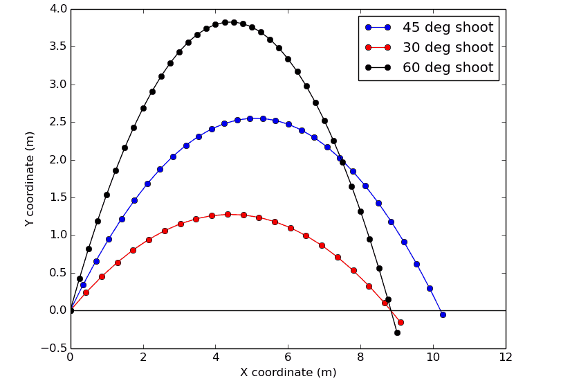
Problem of the missile motion can be solved analytically as well as with the PC. Let’s now check the results displayed above. Taking into account that \dfrac{dv}{dt} = a and \dfrac{dx}{dt} = v one can easily integrate Eqns (1) and get the rules for horizontal and vertical motions:
<br /> \begin{cases}<br /> x(t) = x_0 + v_xt,\\<br /> y(t) = y_0+v_yt-\dfrac{gt^2}{2},\\<br /> \end{cases}
where velocities v_x = v_0\cos\alpha and v_y = v_0\sin\alpha. Excluding time and setting x_0=y_0=0 for simplicity we obtain an equation for missile trajectory:
y(t) = x\tan\alpha – \dfrac{gx^2}{2v^2\cos^2\alpha} (2)
Substituting values used in the code x = 10 m, v = 10 m/s and \alpha = 45^{\circ} one obtains y(10) = 0.2 m which coincides with result obtained numerically.
The integration method used is not suitable for any problem, but very simple for coding and understanding basic principles. In general case, nonlinear differential equations of arbitrary order are reduced to system of the first order equations solved simultaneously via any appropriate integration scheme like Runge-Kutta, BDF or Adams with tolerance control.